I had a access to a smartboard, so I had all of the students gather around (away from their computers) to go over the concepts from Day 1 in a group format. I asked them answer questions about menus and specific purposes of certain functions.
Map Projections
Show a globe and talk about a round-ish earth and what has to happen to made a 2D map of a 3d object.
Talk about how different projections preserve different attributes and are designed for different extents.
Talk about units and how units are associated with a projection/CRS
Zoom in and out with google maps to show the transition from a sphere to a 2d Pseudo-Mercator projection.
Load the 50m_admin_0_countries into qgis. Talk about the ‘on-th-fly’ default and how datasets have a CRS, and the map view can have its own. Lots of math happening behind the scenes…
Set the map view to EPSG: 3857 and talk about disortion. Note the size of Greenland in relation to South America
Set the map view to EPSG: 8857 (Equal Earth) and talk area being preserved. Note the size of Greenland in relation to South America
Choose a few other projections and reproject the map view. Use EPSG codes via the qgis search dialogue in order to alleviate errors at this stage. Choose a polar projection and see the data ‘break’
Getting Data from the Internet
Talk about getting data from the internet and how it will come in various levels of quality, extents, scales and projections.
Adding a WMS basemap layer to QGIS: http://gis.sinica.edu.tw/worldmap/wmts/1.0.0/WMTSCapabilities.xml
Add in the imagery layer and zoom around. this is a crowd-pleaser
Have the students unzip it in the downloads folder, look at the file types, copy it to their Users/Username/data folder and highlight the importance of keeping it organized. Use this oportunity to talk again about data types (.shp, .geodb, .gpkg, .csv)
Geoprocessing Fundamentals
Buffers: load a polyline layer (I chose a trails dataset), and create a half-mile buffer dataset. Calculate area of the output polygons via Vector>Analysis>Basic Statistics…
Clip: Select a county from the Montana counties dataset, and clip the Montana geology dataset to the the county boundary. Use this opportunity to style the layer, label it, and ask questions about the geology polygons, where are the sedimentary types, where are the igneous?
Editing: Introduce the editor toolbar, memory layers and basic editing tools. Make a rectangle and clip the geology layer to the rectangle. Edit some nodes on an existing dataset. Delete by selection tool, Delete by row selection in attribute table, select by expression, delete selected features. Reinforce the concept of a memory layer vs. saving data to disk.
Symbolization
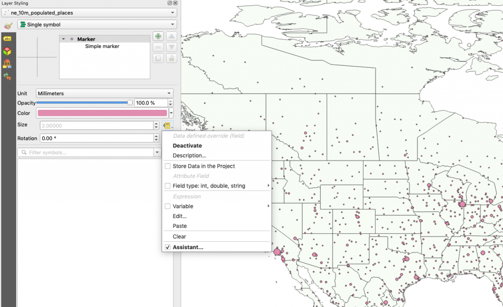
Graduated Symbols: Load ne_10m_states_provinces, ne_10m_populated_places, view the attibute table and have the students locate the field for population on the pop_places dataset.
Use the styling assistant to setuip the graduated symbols:
Layer_styling>simple marker>Size>menu>Assistant…
Source: Choose POP_MAX field
Refresh
Set output sizes from 1 to 10
Collect Field Data
Talk about Field Data collection and the three main geometry types (points, lines, and polygons)
If the students have smartphones, have them install the Input app and have them all login to the same username and password that you have previously setup.
Using the default project, or one that you have setup with that account, head out into the field and have them all collect data, points, lines, and polygons and take some geotagged pictures as well. Have them all sync the data to the public mergin cloud.
Back in the lab, have all of the students install the Mergin plugin via the QGIS Plugins menu.
Have them all login to the same account, load the project locally, and then sync all of the data.
Explore the data that they have collected, look at the attribute tables, and show them how a geotagged photo has the filename in the attribute table and the photo with the matching filename is also stored in the mergin project folder.
On this night, I had to source some custom datasets from the internet that each student would need to complete their project. Give them links if possible so that the student has to download, unzip and organize the data into their project.
Print Composer
Introduce the Print Composer and explain that it is a different window, but linked to the main qgis window.
New Print Layout>Name it for the paper size
Right-Click on the page>Page Properties>Set US Letter Page Size
Add Map
Move tool (layout manipulation)
Move Content Tool (set map extent and scale) #make sure they understand this tool difference
Scale, North Arrow, Title, Legend, Shapes, Attribute Table
Have the students style and print a 8.5×11″ map to the color printer using a selection of the datasets that they have active in qgis (pop_places, geology, etc.)